A bearing that runs today can seize the line next week, and the plain velocity spectrum often shows nothing until the damage is advanced. Envelope analysis reads the low-energy impacts that a damaged race or roller produces, weeks or months before the fault is visible in a normal FFT. After reading this article you can set up an envelope measurement, calculate the bearing fault frequencies, and decide whether the reading justifies a work order.
Why a damaged bearing hides in the ordinary spectrum
A spall on a race or a cracked roller strikes the mating surface each time it passes through the load zone. Each impact is short, so its energy spreads over a wide frequency range, often up to several kilohertz. The impact itself excites structural resonances of the housing, typically between 2 kHz and 20 kHz depending on the machine. The repeating impact rate, usually between 50 Hz and 500 Hz, sits far below these resonances and drowns in noise from unbalance, misalignment, gear mesh and flow turbulence.
The resonances act as mechanical amplifiers. The bearing fault does not change their frequency, but it modulates their amplitude at the fault rate. The spectrum therefore shows resonance peaks whose sidebands sit at the fault frequency, and those sidebands carry very little energy. Envelope analysis shifts the measurement problem: instead of reading the fault frequency directly, you demodulate the amplitude modulation of a resonance band and read the fault rate in a quiet low-frequency range.
This principle is standard practice under ISO 13373, which covers vibration condition measurement and evaluation procedures, and it fits into the monitoring strategy defined in ISO 17359.
The four fault frequencies you must calculate first
Every rolling element bearing produces four characteristic rates. You need the shaft speed, the number of rolling elements, the ball or roller diameter, and the pitch diameter of the bearing. With the shaft frequency f_s in Hz:
- BPFO (outer race) = (N / 2) · f_s · (1 − d / D · cos φ)
- BPFI (inner race) = (N / 2) · f_s · (1 + d / D · cos φ)
- BSF (rolling element) = (D / 2d) · f_s · (1 − (d / D)² · cos² φ)
- FTF (cage) = (1 / 2) · f_s · (1 − d / D · cos φ)
where N is the number of rolling elements, d the rolling element diameter, D the pitch diameter, and φ the contact angle (0 for deep-groove ball bearings). BPFO is usually the highest of the four, so it is the first peak to appear in an envelope spectrum. Use the Bearing Fault Frequency Calculator to get exact values from the bearing designation instead of estimating them.
If the bearing data sheet is missing, measure the geometry from the spare part or read N and approximate d/D from a bearing catalogue. A wrong d/D shifts the predicted frequency by a few percent, which is acceptable; a wrong shaft speed shifts it by the whole ratio, which is not. Confirm the running speed with a tachometer or from the electrical line frequency and the motor slip.
Site procedure for an envelope measurement
Follow this sequence on the machine:
- Confirm the machine is in its normal operating state: same speed, load and temperature as previous readings. Bearing signatures change with load.
- Mount an accelerometer stud-mounted or with a magnet on the bearing housing, as close to the load zone as possible. Stud mounting gives a usable range above 10 kHz; a magnet limits you to roughly 5 kHz.
- Record the raw time waveform at a sampling rate of at least 51.2 kHz for 5 to 10 seconds. Keep the raw file; you can reprocess it later with different bands.
- Inspect the plain spectrum first. Note the shaft rate, any unbalance and misalignment peaks, and the resonance region between 2 kHz and 20 kHz.
- Choose an envelope band that contains a strong resonance peak but avoids gear mesh frequencies and known electrical frequencies (2× line frequency, blade-pass rates). A band 1 kHz to 2 kHz wide is a practical starting point.
- Band-pass filter the raw signal to that band, then demodulate: rectify the signal and low-pass filter it, or use the Hilbert transform. The result is the envelope signal.
- FFT the envelope signal with a frequency resolution fine enough to separate BPFO from shaft rate, typically 400 lines or better over 0 to 500 Hz.
- Compare the envelope spectrum peaks against BPFO, BPFI, BSF and FTF. A real fault shows the fault rate and its harmonics, often with shaft-rate sidebands around BPFI.
- Log the band, the sensor position and the setup with the reading. Trend the same setup at the same point next time.
How to read the envelope spectrum
Judge the pattern, not a single number. Early outer race damage shows one to three harmonics of BPFO with low amplitude. As the fault grows, more harmonics appear, the noise floor between them rises, and the harmonics of shaft rate fade because the fault dominates the modulation. Inner race faults show BPFI with sidebands spaced at the shaft rate, because the fault passes through the load zone once per revolution. Rolling element faults show BSF, often with a 2× BSF component because the defect strikes both races. Cage damage shows FTF, which is a late and serious indication because a failing cage can lead to seizure with little warning.
Envelope amplitude units differ between instruments (g, gE, or demodulated units), so absolute alarm levels are not portable between setups. Trend the amplitude at the fault frequency on the same machine, same point, same band. When the trend rises consistently over two or three measurements, schedule the repair. For the overall machine condition, evaluate the broadband velocity reading against ISO 10816-3 (or ISO 20816-3 for newer installations), which classify machines by power and foundation type and give severity zones A to D. Envelope analysis finds the bearing fault; the ISO zones tell you how the machine as a whole is coping.
Common mistakes that produce false calls
- Enveloping the wrong band. If the band contains gear mesh or a strong discrete tone, the envelope spectrum fills with gear and shaft harmonics. Check the plain spectrum before choosing the band.
- Too coarse frequency resolution. BPFO and its first harmonic can sit within a few hertz of each other at low speeds. Use at least 400 lines over the envelope range.
- Comparing readings taken at different sensor positions or mounting methods. A magnet mount versus a stud mount changes the measured amplitude substantially.
- Ignoring speed variation. A 5 percent speed error moves BPFO by 5 percent, enough to mislabel a peak. Trend frequencies as well as amplitudes.
- Reading electrical noise as a fault. Peaks at exactly 1× and 2× line frequency in the envelope spectrum usually come from the drive, not the bearing.
You can rehearse the interpretation with the Amplitude Modulation and Sideband Simulator and the Time Waveform and FFT Spectrum Simulator before you face a real machine.
Where envelope analysis fits in the maintenance program
Envelope analysis is one layer of a condition monitoring program under ISO 17359. Combine it with overall velocity trending per ISO 10816-3, thermography, and ultrasound for slow-speed or inaccessible bearings. For rotating equipment in general, ISO 18436 defines the competence levels of the people who take and interpret these readings; make sure the analyst is certified for the level of decision you expect them to make. Balancing quality of the machine itself follows ISO 21940-11 and ISO 21940-14; a machine balanced to its tolerance class produces a cleaner spectrum, which makes early bearing signatures easier to see. For fan installations, the airborne noise limits in ISO 14694 matter to the environment but do not affect the bearing measurement.
If you cannot tell whether a peak is a bearing fault or a structural resonance, check the Vibration Fault Spectrum Simulator or run the Why Is My Machine Vibrating? Diagnosis Wizard with your spectrum data.
When to call for an on-site measurement
Call for on-site help when the envelope trend rises but the machine cannot stop, when several bearings show signatures at once, when the speed varies so much that fault frequencies wander, or when you need a phase-referenced measurement to separate a bearing fault from unbalance or misalignment. A field measurement with a 24-bit DAQ, correct sensor mounting and a controlled operating point resolves those cases in one visit. REI Balance performs on-site vibration analysis and field balancing; request a measurement through the contact page at REI Balance field services.